Learning the Effect of Registration Hyperparameters
Andrew Hoopes and Adrian Dalca
Hyperparameter tuning is a time-consuming process in a wide variety of medical image analysis tasks, especially in the context of Deep Learning. In this tutorial we describe a strategy to alleviate challenges of hyperparameter tuning, and while we specifically focus on image registration, these concepts apply broadly.
Deformable registration is a common medical imaging technique that computes a dense transform (a deformation field) to accurately align two images. In more recent years, learning-based implementations of image registration have gained significant popularity.
However, hyperparameter tuning in learning-based registration involves training many separate models with various hyperparameter values, potentially leading to suboptimal results. HyperMorph addresses this inefficiency and removes the need to tune important registration hyperparameters during training by learning the effects of hyperparameters on deformation fields.
Generally, the HyperMorph strategy involves a secondary network, called a hypernetwork, that learns to predict the weights of a primary network for a given set of hyperparameter values. In effect, this strategy trains a single, rich model that enables rapid, fine-grained discovery of hyperparameter values from a continuous interval at test-time.
In this tutorial, we’ll develop and train a HyperMorph model to learn the effect of a common registration hyperparameter. This walk-through assumes some basic knowledge of learning-based image registration techniques, and some prior experience with the Keras and TensorFlow libraries might be useful. While the HyperMorph strategy can be implemented for any network, here we build off the open-source VoxelMorph registration library. For further information, there are plenty of useful resources, including papers and tutorials, on the VoxelMorph GitHub page. The first section of this tutorial builds loosely off the main VoxelMorph tutorial.
Setup
We’ll use TensorFlow 2.4 as well as the neurite and voxelmorph open-source python packages. The hypernetwork-based features are available in the development versions from GitHub.
pip install git+https://github.com/adalca/pystrum.git@dev
pip install git+https://github.com/adalca/neurite.git@dev
pip install git+https://github.com/voxelmorph/voxelmorph.git@dev
Let’s import all of our modules, and make sure to disable TensorFlow’s eager execution, which is currently incompatible with the hypernetwork training framework.
import numpy as np
import neurite as ne
import voxelmorph as vxm
import tensorflow as tf

tf.compat.v1.disable_eager_execution()
Data
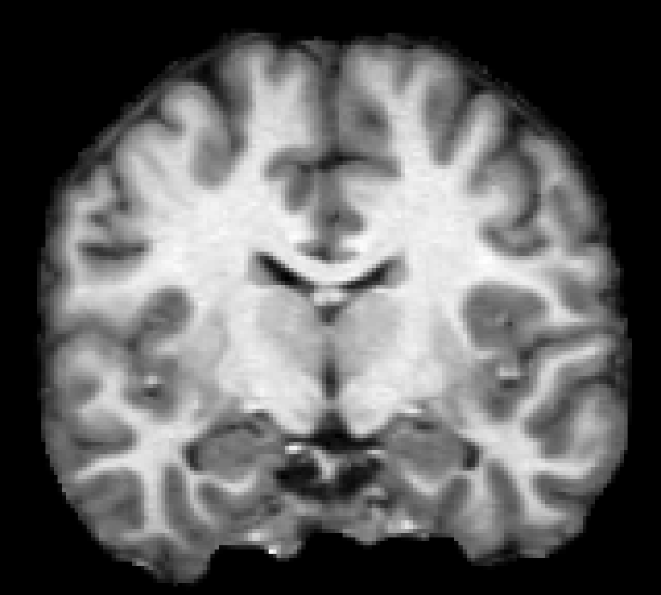
Our goal is to align pairs of brain MR slices across a set of subjects gathered from the public OASIS dataset. This sample subset consists of 414 2D images, which can be loaded directly from neurite.
images = ne.py.data.load_dataset('2D-OASIS-TUTORIAL')
Each image is conformed to the shape (height × width × channels) where channels = 1, and the pixel-data is normalized between 0 and 1. We can visualize the first image in our dataset with the ne.plot.slices() function.
image = images[0].squeeze()
image_shape = image.shape
ne.plot.slices(image)
We need to split the data evenly into training, validation, and test sets, each with 138 images.
train_data, validate_data, test_data = np.array_split(images, 3)
Training a registration network
To start, let’s train a standard VoxelMorph registration network (with hard-coded hyperparameters) that learns to align our sample image data. We won’t cover the details of VoxelMorph in this tutorial, but include just enough information to enable us to illustrate the importance of the hypernet strategy. Detailed VoxelMorph-specific tutorials are available online.
We’ll use the vxm.networks.VxmDense class, which subclasses a Keras Model and requires some information about the input image shape.
model = vxm.networks.VxmDense(image_shape, int_steps=0)
This VoxelMorph network is essentially a simple U-Net that takes as input an image pair (a moving and fixed image) and predicts a 2D deformation field that aligns the input moving image with the fixed target. By setting int_steps to 0, we’ve disabled diffeomorphic fields. By default, our configured model outputs two tensors: the first is the moved image (the moving image warped by the displacement field) and the second is the deformation field itself.
Now, let’s configure our loss functions, which are a focus of this tutorial. In registration, deformation fields are generally optimized with a multi-term loss that (1) maximizes the similarity between the moved and fixed images and (2) enforces some regularization on the field to prevent anatomically inaccurate displacements. In this tutorial, we’ll use MSE as an image similarity metric, and we’ll regularize (or smooth) the deformation field by minimizing the gradient around neighboring vectors.
The relative weight of these two loss terms is balanced by an important hyperparameter λ, which can vary (between 0 and 1 for purposes of this tutorial). The value chosen for λ can have substantial effects on the final registration accuracy (and has been a focus of ongoing research in the last few decades), but for now, we’ll use a hard-coded λ = 0.5.
lambda_weight = 0.5
image_loss = lambda yt, yp: vxm.losses.MSE(0.1).loss(yt, yp) * (1 - lambda_weight)
gradient_loss = lambda yt, yp: vxm.losses.Grad('l2').loss(yt, yp) * lambda_weight
losses = [image_loss, gradient_loss]
We need to configure a generator to produce data for each training step. At each iteration, we sample two random images, representing the input moving and fixed images, from the training set. In this tutorial, we’ll use a batch size of one and start with a standard VoxelMorph generator:
def voxelmorph_generator(data):
    image_shape = data.shape[1:]
    ndims = len(image_shape)
    # the gradient loss is computed entirely on the predicted deformation,
    # so the reference data for the second model output can be ignored and
    # we can just provide an image of zeros
    zeros = np.zeros([1, *image_shape, ndims], dtype='float32')
    while True:
        # for each training iteration, grab a random pair of images to align
        moving_image = data[np.random.randint(len(data))][np.newaxis]
        fixed_image = data[np.random.randint(len(data))][np.newaxis]
        inputs = [moving_image, fixed_image]
        outputs = [fixed_image, zeros]
        yield (inputs, outputs)
Now that we’ve configured the losses and data generation, we can compile and train our model using the Adam optimizer. Let’s run the training for 500 epochs.
model.compile(optimizer=tf.keras.optimizers.Adam(lr=1e-4), loss=losses)
gen = voxelmorph_generator(train_data)
history = model.fit_generator(gen, epochs=500, steps_per_epoch=100)
This step should take about 5 minutes on a GPU. While it’s unlikely that the model has properly converged at this point, it should be sufficient for the sake of this tutorial. Make sure to train your models fully (until the training or validation loss stops going down) under normal circumstances!
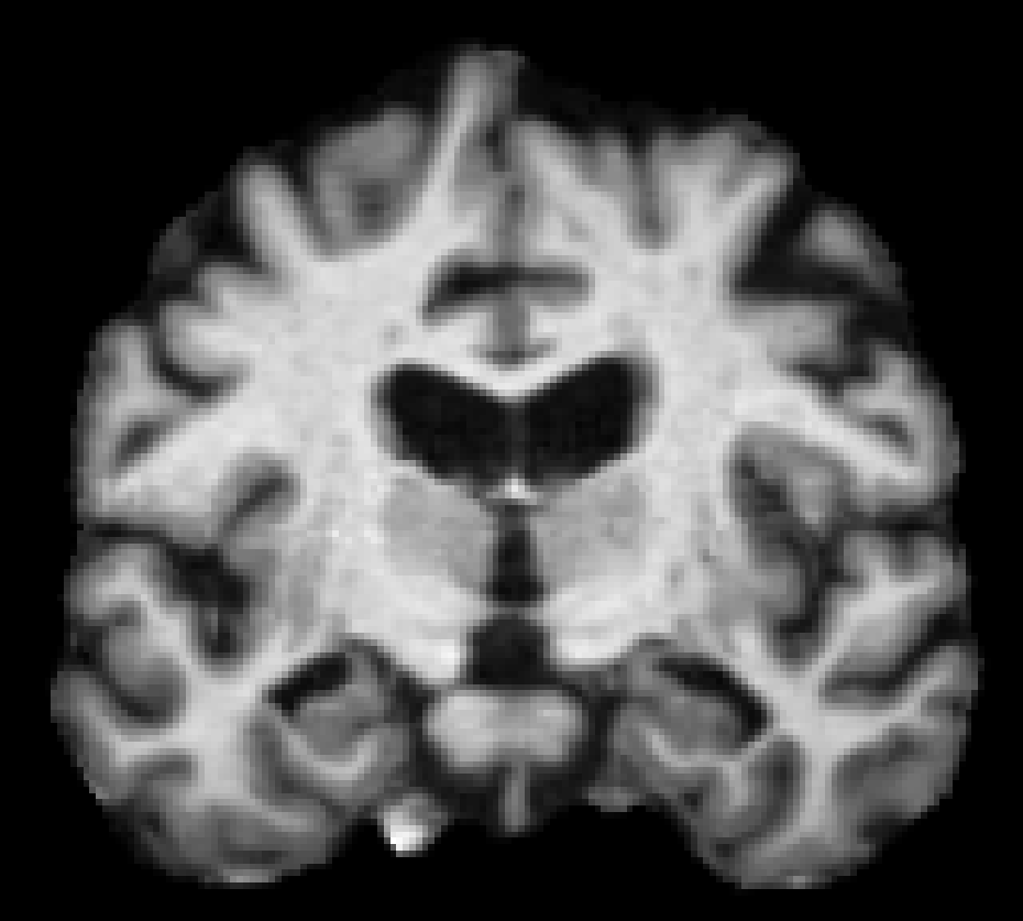
We can evaluate the model accuracy by predicting registrations across our validation images. Let’s grab an arbitrary moving and fixed image pair and visualize the resulting alignment.
# predict the registration
moving_image = validate_data[2][np.newaxis]
fixed_image = validate_data[11][np.newaxis]
moved_image, warp = model.predict([moving_image, fixed_image])

# visualize the result
slices = [moving_image, fixed_image, moved_image]
titles = ['Moving', 'Fixed', 'Moved']
ne.plot.slices(slices, titles=titles)
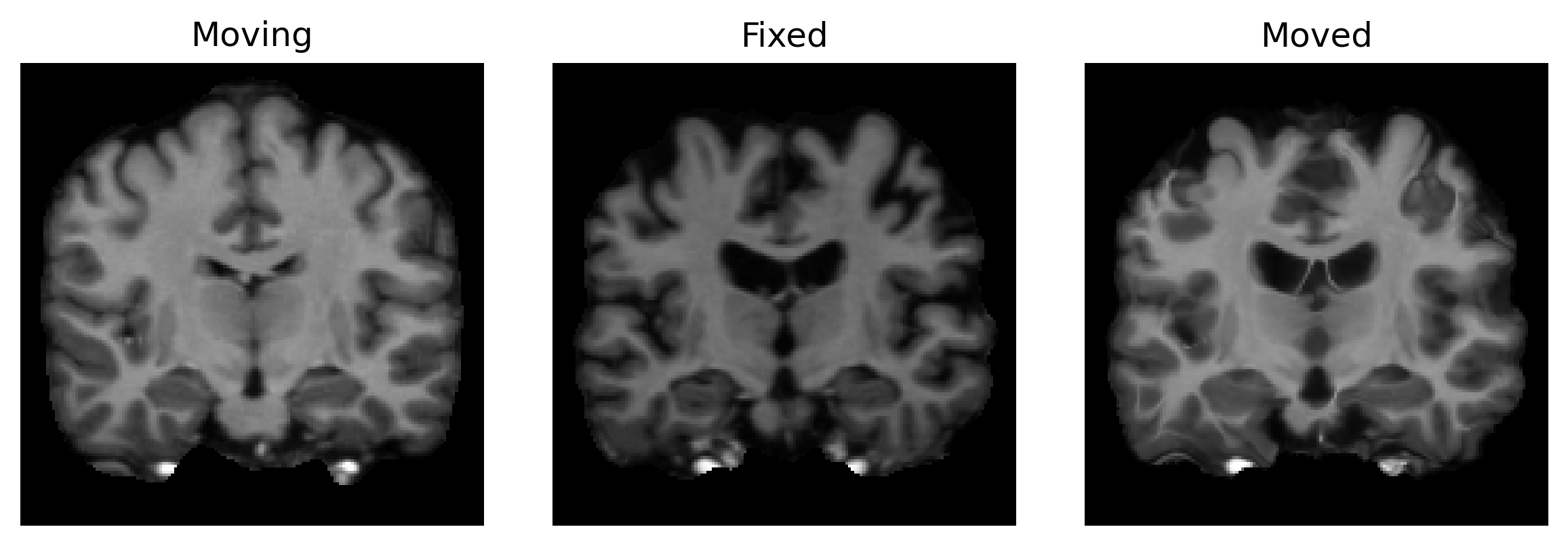
Not bad... but could the result be even better if we trained our model for a different value of λ? This is often a crucial decision when using a registration model.
The traditional way to answer this question is by training and evaluating a large series of models for different values of the hyperparameter. However, this can be incredibly tedious and time consuming, especially when working with large 3D networks that might take days or even weeks to converge!
Training a HyperMorph model
To alleviate this burden, we can instead train a single HyperMorph model to learn the effect of the hyperparameters that we care about. This way, we can evaluate the impact of λ entirely at test time, without having to train multiple models. Let’s try it out!
Remember, HyperMorph is implemented by training a hypernetwork that predicts the weights of a target network. So, in our case, we want to configure a fully-connected network that takes a single λ value as input and outputs the weights of our primary VoxelMorph registration network. Let’s build a four-layer hypernetwork using a series of Dense Keras layers, and integrate it with our registration model via the hyp_model parameter.
hp_input = tf.keras.Input(shape=[1])
x = tf.keras.layers.Dense(32, activation='relu')(hp_input)
x = tf.keras.layers.Dense(64, activation='relu')(x)
x = tf.keras.layers.Dense(128, activation='relu')(x)
x = tf.keras.layers.Dense(128, activation='relu')(x)
hypernetwork = tf.keras.Model(hp_input, x, name='hypernetwork')

model = vxm.networks.VxmDense(image_shape, int_steps=0, hyp_model=hypernetwork)
Important: in this new model, the only trainable weights are in the hypernetwork. For tutorial purposes, we’ve coded the dense hypernetwork from scratch, but it is also available directly via the vxm.networks.HyperVxmDense model class, which configures the hypernetwork architecture behind the scenes.
We’re almost ready to start training our HyperMorph model, but first we need to modify the losses and data generator a bit. During training, we want to make sure that the input λ value is properly used in the loss to facilitate appropriate gradients that are dependent on the hyperparameter. Let’s reconfigure our loss functions by setting lambda_weight equal to the hyperparameter input tensor defined above.
lambda_weight = hp_input
image_loss = lambda yt, yp: vxm.losses.MSE(0.05).loss(yt, yp) * (1 - lambda_weight)
gradient_loss = lambda yt, yp: vxm.losses.Grad('l2').loss(yt, yp) * lambda_weight
losses = [image_loss, gradient_loss]
Also, since our new model also accepts an input hyperparameter value, we’ll need to extend the generator to randomly sample a λ value between 0 and 1 for each training iteration. We can just build off of our existing generator function here.
def hypermorph_generator(data):
    # initialize the base image pair generator
    gen = voxelmorph_generator(data)
    while True:
        inputs, outputs = next(gen)
        # append a random λ value to the input list
        inputs = (*inputs, np.random.rand(1, 1))
        yield (inputs, outputs)
We’re ready to optimize the HyperMorph model. This time, we will train the network for a little longer.
model.compile(optimizer=tf.keras.optimizers.Adam(lr=1e-4), loss=losses)
gen = hypermorph_generator(train_data)
history = model.fit_generator(gen, epochs=1000, steps_per_epoch=100)
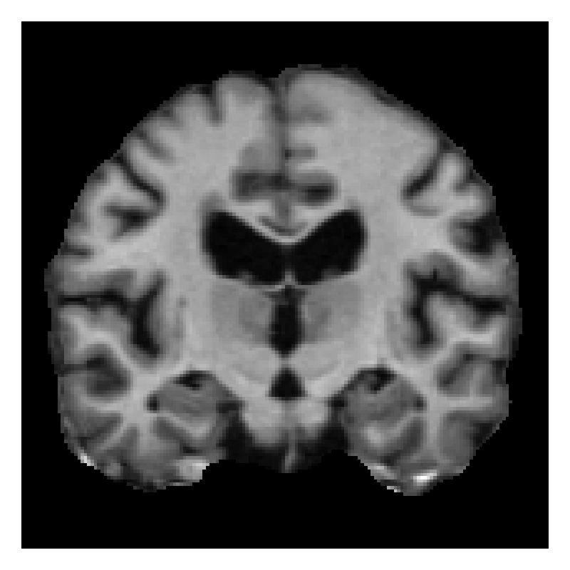
Once trained, we now have a model that can predict corresponding deformation fields for any value of λ! Let’s visualize the predicted alignments for a few different regularization weights.
lambdas = np.linspace(0, 1, 5).reshape((-1, 1))
slices = [model.predict([moving_image, fixed_image, hyp])[0] for hyp in lambdas]
titles = ['λ = %.2f' % hyp for hyp in lambdas]
ne.plot.slices(slices, titles=titles)
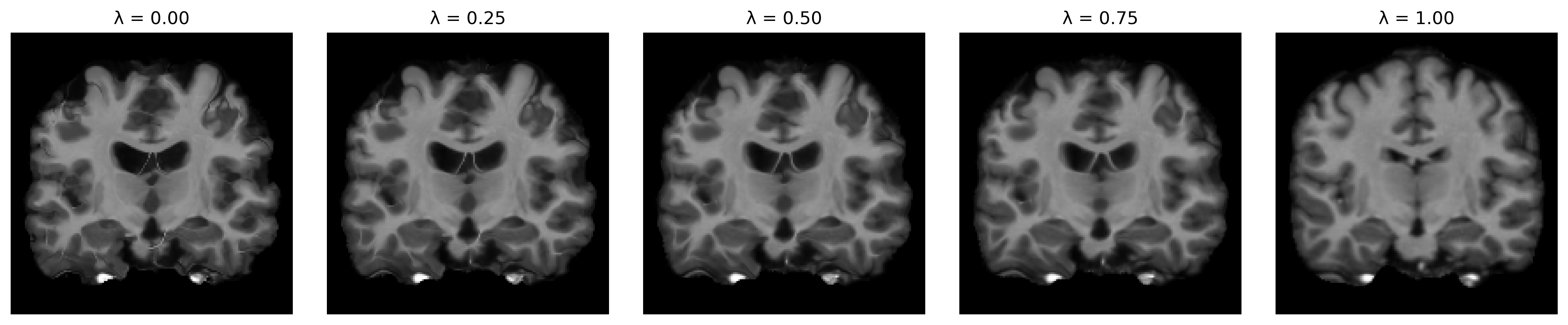
Here, we evaluated the model for a single image pair, but in practice, we can effectively choose ideal values for λ across a set of validation pairs, evaluating registrations either visually or via some registration metric, like the overlap of corresponding anatomical segmentations.
Takeaways
The HyperMorph strategy facilitates fast hyperparameter search. Importantly, it also enables the ability to vary the hyperparameter at test time. This is critical since the often overlooked reality is that there’s no such thing as “one true optimal” hyperparameter value. For example, the optimal regularization weight can differ largely across dataset, modality, task, and even anatomical region, so it’s essential to have the ability to adapt hyperparameters on the fly.
Furthermore, while this tutorial focused on registration, the underlying strategy can be adapted to countless learning-based applications, far beyond the domain of registration or even medical imaging! If you’re interested in experimenting with hyper-architectures in TensorFlow, the neurite library has Keras layers for easy hypernetwork integration. If you’d like a closer look at how HyperMorph is implemented, check out the VoxelMorph source code.
We hope this tutorial helps you try out hypernetworks for your own problem!